Ever wondered what happens to image quality when you remove a photo’s background? Separating subjects (like a dog) from their surroundings doesn’t just change appearance – it transforms how we measure image quality itself.
Our study analyzed dog photos before and after background removal, revealing surprising results. Segmentation typically makes the subject appear sharper and the image more uniform. However, it often reduces “naturalness” scores – the technical metrics suggest these isolated subjects look less like real-world scenes.
This counterintuitive finding matters for how we process and enhance digital images. Let’s explore the science behind what happens when your subject stands alone.
Description of the analyzed metrics
When analyzing images, we need objective ways to measure their quality. Below is a brief overview of key metrics that help quantify different aspects of image clarity, sharpness, and naturalness.
- Laplacian methods. The “edge detectives” that highlight rapid brightness changes, excellent for detecting focus shifts.
- Tenengrad. Measures edge crispness – sharper images have stronger edges and higher values.
- Image entropy. Assesses detail diversity – sharp images are like bustling cities with high entropy; blurry ones are like foggy mornings with low entropy.
- Dynamic range. The span between darkest and lightest points – wider ranges preserve more details in both shadows and highlights.
- Gradient contrast. Captures clear, well-defined boundaries between objects – the sharp edge of a mountain against the sky.
- Blockiness. Measures those chunky squares in compressed images – segmentation often reduces this by removing background areas.
- FWHM. Estimates blur by measuring transition width at edges – smaller width means sharper edges.
- GLCM features. Statistical texture analysis examining contrast, homogeneity, energy, and correlation patterns.
- Congruency. Evaluates gradient consistency across images – higher values indicate more uniform gradients.
- JNB. A human-perception-based blur measure – low values mean the image appears sharp to viewers.
- NIQE. Compares image statistics to “natural” photo models – removing backgrounds can make images seem less natural.
🧐 For more details on these metrics and segmentation effects, see our full guide: Understanding Image Quality Metrics: A Comprehensive Guide
Adaptation of metrics for segmented objects
Traditional image quality metrics are designed with whole-frame analysis in mind. But what happens when we’re only interested in the main subject – like a dog – and not the background?
The standard approach would evaluate everything in the frame, but we’ve tweaked these metrics to consider only what’s happening within our “star” (the segmented object).
After segmentation, the background might be artificially blank (like a black backdrop) or contain distracting elements (noise, textures, or photobombers). These can skew our measurements. To solve this problem, we modified all the classic metrics to analyze only what’s inside the object’s boundaries.
In some cases, we went a step further. To prevent the sharp edge between object and empty background from influencing our measurements, we replaced the background with the object’s median brightness value. This is similar to how photographers use neutral backgrounds for product photography – it lets us evaluate the subject without distractions.
These adaptations ensure we’re measuring what matters: the quality of our main subject, not the artificial conditions created by segmentation.
1. Variance of Laplacian (VoL)
Classical definition: VoL(I) = Var(∇²I) where ∇²I is the Laplacian of the image.
Adaptation for object-only evaluation: VoL(I,M) = Var((∇²I)·M) where M is the binary mask of the object.
This prevents background pixels from artificially lowering variance. Calculated only within the object mask (M). This ensures VoL reflects only the sharpness of the dog’s fur and contours.
2. Dynamic range (DR)
Computed only within the mask. This prevents the black background from trivially setting the minimum to 0.
Classical definition: DR(I) = max(I) – min(I)
Adaptation: DR(I,M) = max(I·M) – min(I·M) ensuring only object pixels contribute to the intensity spread.
3. Gradient-based metrics (Tenengrad, gradient contrast)
Averaged only over object pixels. This avoids artificial inflation from gradients at the object-background boundary.
Classical gradient contrast: GC(I) = (1/HW) ∑(x,y) √(Gx(x,y)² + Gy(x,y)²)
Object-focused adaptation: GC(I,M) = (1/|M|) ∑(x,y)∈M √(Gx(x,y)² + Gy(x,y)²)
Tenengrad: T(I,M) = (1/|M|) ∑(x,y)∈M (Gx(x,y)² + Gy(x,y)²)
Where Gx, Gy are Sobel gradients and ∣M∣ is the number of object pixels. This prevents spurious gradients at the object–background boundary from inflating sharpness.
4. Blockiness
Averaged only within the object mask to prevent strong jumps at the object–background boundary from being misinterpreted as compression artifacts.
Vertical block transitions: Bᵥ(I) = (1/HW) ∑ₓ,ᵧ |I(x,y) – I(x,y-1)|
Object-only adaptation: B(I,M) = [∑(x,y)∈M |I(x,y) – I(x-1,y)| + |I(x,y) – I(x,y-1)|] / |M| excludes artificial jumps caused by background.
5. FWHM
The brightness profile is computed by summing intensities only within the mask for each column.
Profile along x-axis: P(x) = ∑ᵧ I(x,y)
Object-only adaptation: Pₘ(x) = ∑ᵧ I(x,y)·M(x,y)
6. GLCM features
The background was replaced with the median intensity value of the object before calculating the co-occurrence matrix. This prevents the artificial “object-to-background” transitions from dominating the texture statistics.
Classical definition: GLCM(i,j) = ∑ₓ,ᵧ 𝟙(I(x,y) = i ∧ I(x+Δx,y+Δy) = j)
Adaptation with median background replacement: I'(x,y) = { I(x,y), if (x,y)∈M ; median(I·M), if (x,y)∉M
GLCM is computed on I′ to avoid skew from artificial background pixels.
7. Congruency
The background was replaced with the object’s median value to prevent sharp mask boundaries from distorting the phase spectrum.
8. JNB
The median gradient and subsequent calculations were performed only within the object mask: JNB(I) = #{(x,y) : G(x,y) < T} / #{(x,y)}
Object-only adaptation: JNB(I,M) = #{(x,y) ∈ M : G(x,y) < Tₘ} / |M|
9. NIQE
The background was replaced with the object’s median value to create a more statistically “natural” patch for evaluation, rather than using a stark black background
This adaptation ensures that the metrics reflect the properties of the object itself (texture, edges) and are not skewed by segmentation artifacts.
Two approaches for metric computation
1. Metrics computed ONLY within segmented region (using mask):
- Variance of Laplacian, Dynamic Range, Gradient Contrast, Tenengrad, Blockiness, FWHM, JNB
- These metrics analyze properties specifically within the detected object boundaries
- We use direct pixel masking to isolate the object region
2. Metrics computed on ENTIRE image with background normalization:
- GLCM, Congruency, NIQE
- Background is replaced with object’s median value to avoid artificial edges/textures
- Why not black background? → Black creates sharp artificial edges that distort texture analysis and frequency domain metrics
- Why not cropping? → Cropping changes image dimensions and context, making metrics inconsistent across different images
- Normalization to [0,1] range is applied for NIQE as required by the algorithm
Key insight: We avoid black background because it introduces artificial high-frequency components that corrupt texture analysis (GLCM) and frequency-domain metrics (Congruency, NIQE). Using the object’s median value for background creates smoother transitions while preserving the original image structure.
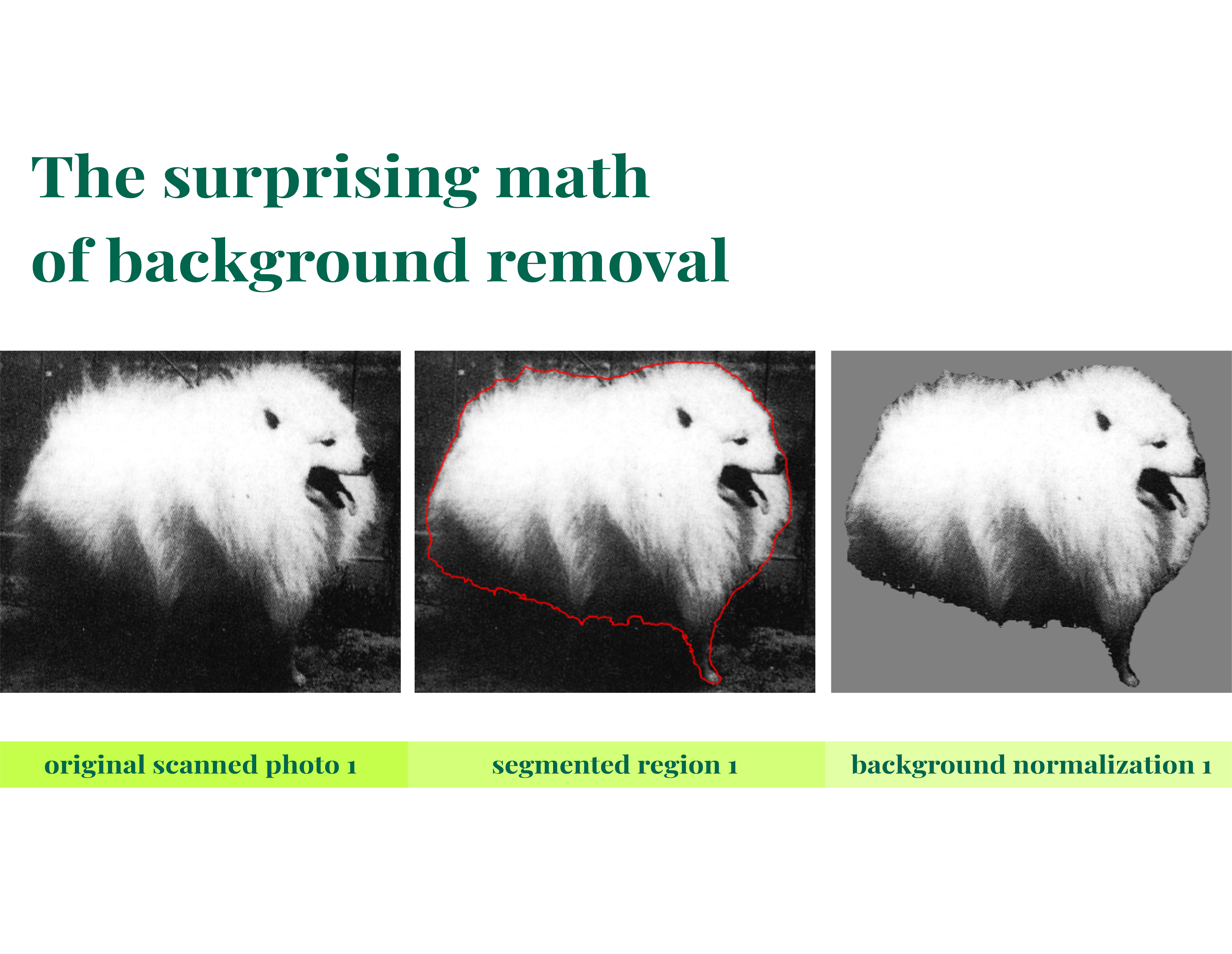
| Original photo |


| For metrics computed ONLY within segmented region (using mask) |


| For metrics computed on ENTIRE image with background normalization |


Comparison of results and experimental data
However, in cases where the background contained sharp details (e.g., textures), Laplacian and Tenengrad could decrease after background removal, as the background provided the majority of sharp edges.
Here are the results we got and the changes in metrics we observed:

- variance_of_laplacian ↑ (2475 → 2858): the dog became sharper, the background was interfering.
- entropy = (0.898 → 0.898): no changes.
- dynamic_range = (255 → 255): the background did not affect it.
- gradient_contrast ↑ (101 → 103): local variations became slightly more pronounced.
- tenengrad ↑ (19959 → 21379): sharpness on the subject is higher.
- blockiness ↓ (27 → 13): segmentation removed sharp background transitions.
- fwhm ↓ (0.88 → 0.72): the image appears slightly more blurred in the segment.
- GLCM contrast ↓ (459 → 310): loss of diverse textures from the background.
- GLCM homogeneity ↑ (0.19 → 0.59): the image became more uniform.
- energy/ASM significantly ↑: segmentation removed noise → more structure.
- correlation ≈ approximately the same (0.97 → 0.96).
- congruency ↑ (0.28 → 0.32): more consistent gradients.
- jnb ≈ approximately the same (0.29 → 0.27).
- niqe ↑ (7.67 → 7.85): subjective quality is worse because without the background, the image looks “unnatural.”
Conclusion: segmentation provided gains in sharpness and uniformity but worsened perceptual metrics (NIQE, FWHM).

- variance_of_laplacian ↑ (38 → 99): the dog is more defined.
- entropy = (0.86 → 0.86).
- dynamic_range = (255 → 255).
- gradient_contrast ↑ (11 → 19): more local contrast on the dog.
- tenengrad ↑ (502 → 1015): higher sharpness.
- blockiness ↓ (2.60 → 2.46): slight improvement.
- fwhm ↓ (0.99 → 0.34): stronger blur on the segment.
- GLCM contrast ↓ (6.7 → 3.1): background provided texture diversity.
- GLCM homogeneity ↑ (0.62 → 0.91): the dog is smoother.
- energy/ASM significantly ↑ (0.07 → 0.86): became more structured.
- correlation ↓ (0.999 → 0.993).
- congruency ≈ approximately the same (0.30 → 0.32).
- jnb ↑ (0.18 → 0.46): perception of sharpness by JNB is better.
- niqe ↑ (10.77 → 13.97): quality is worse, background was important for “naturalness.”
Conclusion: higher sharpness, more uniform texture, but NIQE ruined the result due to the absence of background.

- variance_of_laplacian ↓ (619 → 388): lower sharpness.
- entropy = (0.89 → 0.89).
- dynamic_range = (248 → 248).
- gradient_contrast ↑ (22 → 25): local contrast increased.
- tenengrad ↑ (1022 → 1587): dog’s sharpness is higher.
- blockiness ↓ (11 → 4): segmentation smoothed transitions.
- fwhm ↓ (0.99 → 0.50): worse subjective clarity.
- GLCM contrast ↓ (65 → 22): loss of background textures.
- GLCM homogeneity ↑ (0.23 → 0.74): the dog is more uniform.
- energy/ASM sharply ↑ (0.02 → 0.64).
- correlation ↓ (0.98 → 0.96).
- congruency ↑ (0.24 → 0.32).
- jnb ↓ (0.21 → 0.20): almost no changes.
- niqe ↑ (6.29 → 6.42): quality is worse.
Conclusion: segmentation provided more sharpness on the subject but reduced the overall quality perception (NIQE, FWHM, Laplacian).

- variance_of_laplacian ↓ (593 → 255): lower sharpness.
- entropy = (0.92 → 0.92).
- dynamic_range ↓ (220 → 202): smaller range, the background provided diversity.
- gradient_contrast ↓ (48 → 33): detail level dropped.
- tenengrad ↓ (4656 → 2508): worse sharpness.
- blockiness ↓ (12.7 → 4.0): fewer artifacts.
- fwhm ↓ (0.99 → 0.49): the dog appears more blurred.
- GLCM contrast ↓ (93 → 39): background provided diversity.
- GLCM homogeneity ↑ (0.19 → 0.74): the dog is smoother.
- energy/ASM significantly ↑ (0.01 → 0.64).
- correlation ↓ (0.97 → 0.95).
- congruency ↑ (0.25 → 0.29).
- jnb ↓ (0.22 → 0.11): worse perception of sharpness.
- niqe ↓ (6.85 → 6.13): better perception (!) — the background was interfering.
Conclusion: technical sharpness is worse, but perceptual quality (NIQE) improved — the background was degrading perception.
Now, let’s get to analyzing the results:
1. GLCM contrast
In all cases, a noticeable decrease in this parameter was observed (e.g., 459 → 310, 93 → 39, etc.). Removing background areas eliminates texture diversity (background “grain,” patterns), making the image less “contrasty” in a textural sense.
2. GLCM homogeneity and energy/ASM
These always increased (e.g., Homogeneity 0.19 → 0.59, Energy 0.02 → 0.64 for one of the images). This is expected: by removing the background with irregular noise, the remaining object has a more uniform texture.
Roughly speaking, the image becomes more “homogeneous” and “structured”.
3. Blockiness
Decreased in all cases (e.g., 27 → 13, 12.7 → 4.0). This is because the background, especially if compressed, contains block artifacts. Segmentation removes these areas, so “blockiness” in the remaining image noticeably decreases.
Blocking artifacts are easily detectable by humans and should be detectable without a reference. Low blockiness values after segmentation indicate a smoother appearance of the object.
4. FWHM
In most cases, a decrease was observed (0.99 → 0.72, 0.99 → 0.49, etc.), which corresponds to the perception of a more blurred area. A smaller width at half maximum means a sharper brightness peak.
A decrease in FWHM after segmentation indicates that the local edges of the object became less sharp (i.e., subjectively more “blurred”) due to the absence of background contrast.
5. JNB
Changed insignificantly. In many cases, its changes were small (0.29 → 0.27, 0.21 → 0.20, etc.), showing that the relative “noticeable blurriness” of the object practically did not change. In one case (2nd image), JNB noticeably increased (0.18 → 0.46), indicating that after segmentation the object became subjectively sharper.
This aligns with the idea that JNB reflects human perception of sharpness.
6. NIQE
Almost always worsened (i.e., the number increased) after background removal: quality “decreased.” For example, NIQE 7.67 → 7.85, 10.77 → 13.97, 6.29 → 6.42 in three out of four cases. This corresponds to the fact that isolating an object makes the image statistically less “natural”.
An exception was the last example: there the background was very “noisy” and unnatural, so its removal decreased NIQE (6.85 → 6.13), i.e., increased subjective quality. This emphasizes that the background is important for the perception of scene naturalness, and NIQE reflects precisely the naturalness of statistics.
Thus, segmentation provides benefits in terms of object sharpness and homogeneity, but often degrades metrics related to quality perception and textural diversity. This is evident in all considered examples.
This is why we observe an increase in sharpness on the object. However, if the background contained texture or sharp elements, Laplacian could decrease (the background provided the main “energy” of the edges) – this is a rare but expected case.
Key insights
Loss of textural diversity
GLCM metrics vividly illustrate the effect of detail removal: we always see a decrease in contrast and an increase in homogeneity/energy. Segmentation removes background elements that previously contributed unique brightness combinations.
As follows from the definition, high GLCM-contrast means strong texture variations, and high GLCM-homogeneity/ASM means very repetitive, smooth patterns. After segmentation, the object becomes more “uniform,” resulting in low contrast and high homogeneity.
Block compression artifacts
The consistent decrease in blockiness confirms that background removal eliminates compression artifacts. In our experiments, the background likely contained smoothed patches or blocks (especially on a uniform background). Removing the background resulted in a smooth object, as seen by the drop in the blockiness metric.
Quality perception (NIQE)
An increase in NIQE indicates a violation of the naturalness of the picture. NIQE is built on the statistics of natural scenes, and an isolated object rarely corresponds to these statistics. Thus, although the technical sharpness of the object increases, the image without a background looks “unscientific” and subjectively worse (which the metric captures).
Only in the case where the background was clearly extraneous noise did its removal improve the statistics: NIQE decreases, quality increases. This underscores that a low NIQE corresponds to a more “realistic” appearance according to the model of natural images.
Summary classification of metric changes
After diving into the mathematical details, let’s step back and see the bigger picture. Here’s how segmentation reshapes our perception of image quality at a glance:
| Always improve (after segmentation) | Usually worsen | Case-dependent |
| Blockiness – sharp block transitions of the background are eliminated. GLCM Homogeneity and Energy/ASM – the object becomes more homogeneous. | NIQE – the image falls outside the statistics of a “natural scene”. GLCM Contrast – texture diversity decreases. FWHM – the subjective blurriness of edges increases. | Variance of Laplacian, Tenengrad, JNB – if the background is less sharp, they increase on the object; if the background is sharper, they may decrease. This corresponds to the fact that these metrics measure focus on sharp boundaries. |
This situation is common in image processing: improvement in technical sharpness metrics does not always mean an improvement in visual perception or scene realism. Our observations confirm the need to balance these indicators when developing segmentation and post-processing algorithms.
Conclusion
Understanding how segmentation affects image metrics reveals a fascinating trade-off: isolating subjects improves technical aspects like sharpness and uniformity while potentially sacrificing perceived naturalness. This insight helps photographers and developers make better choices about when to remove backgrounds and how to interpret quality measurements in today’s image-processing landscape.
Leave a Reply